Demand restrictions
Demand restrictions are a common concept in water resource models. When the state of a water resource is poor (for example, lower than normal reservoir levels) demand restrictions may be imposed on customers in order to reduce the likelihood of a failure to supply.
The demand at a given timestep can be represented using the equation below,
where \(d\) is the final demand to be calculated, \(d_{mean}\) is the baseline demand, \(p\) is the annual profile and \(s\) is the demand restriction (e.g. 5%).
The code snippets that follow belong in the "parameters": {} section of the model document (except for the node at the end).
The baseline demand is specified as a constant (this is often the mean annual demand).
"demand_baseline": {
    "type": "constant",
    "values": 50
}
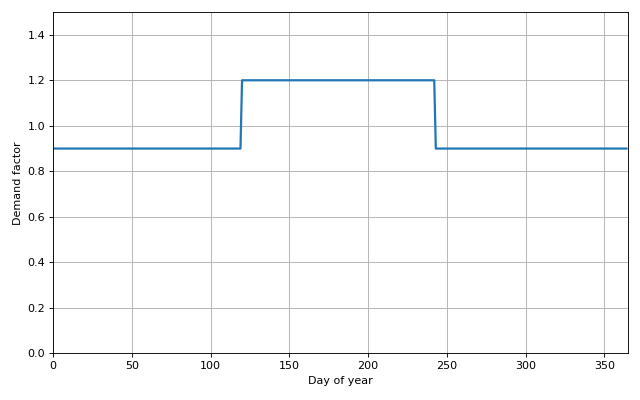
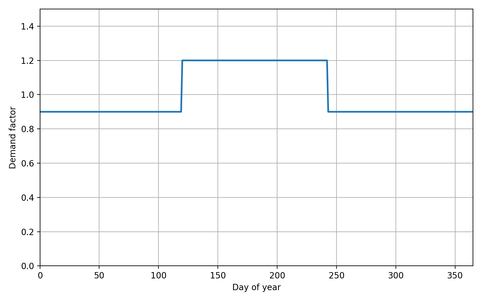
A daily or monthly profile can be used to vary the demand throughout the year. In the example below the demand in May - August is 1.2x the baseline demand, with the rest of the year at 0.9x the baseline, forming the common “top hat” profile (illustrated below).
"demand_profile": {
    "type": "monthlyprofile",
    "values": [0.9, 0.9, 0.9, 0.9, 1.2, 1.2, 1.2, 1.2, 0.9, 0.9, 0.9, 0.9]
},
(Source code, png, hires.png, pdf)

The demand restriction level describes the level of restrictions as an integer, where 0 means no demand restrictions, level 1 (L1) is some restriction (or perhaps just publicity), level 2 (L2) more severe restrictions, and so on. The specifics will depend on the system being modelled. This is represented in Pywr using the ControlCurveIndexParameter. IndexParameter return an integer to be used as an index, rather than a decimal value.
The demand restriction level is often related to the storage of strategic reservoirs in relation to a control curve (the expected reservoir volume at a given time of the year). The example below two demand restriction levels are defined (and implicitly a L0) based on the volume in the "Central Reservoir" storage node. L1 is defined as 80% of full, L2 as 50% of full. Control curves are commonly more complicated, as the expected level of a reservoir is usually lower in the summer than it is in the winter.
"demand_restriction_level": {
    "type": "controlcurveindex",
    "storage_node": "Central Reservoir",
    "control_curves": [
        "level1",
        "level2"
    ]
},
"level1": {
    "type": "constant",
    "values": 0.8
},
"level2": {
    "type": "constant",
    "values": 0.5
},
The demand restriction factor is determined by indexing an array of possible restriction profiles with the demand restriction level (i.e. index). In the example below the list of profiles ("params") corresponds to the L0, L1 and L2 profiles respectively. At L0 a constant factor 1.0 is used to represent no restrictions. At L1 there is a 10% reduction in demand (0.90 as a factor) during the summer months and a 5% reduction elsewhere (0.95). At L2 there are further reductions to 75%/80%.
"demand_restriction_factor": {
    "type": "indexedarray",
    "index_parameter": "demand_restriction_level",
    "params": [
        {
            "type": "constant",
            "values": 1.0
        },
        {
            "type": "monthlyprofile",
            "values": [0.95, 0.95, 0.95, 0.95, 0.90, 0.90, 0.90, 0.90, 0.95, 0.95, 0.95, 0.95]
        },
        {
            "type": "monthlyprofile",
            "values": [0.8, 0.8, 0.8, 0.8, 0.75, 0.75, 0.75, 0.75, 0.8, 0.8, 0.8, 0.8]
        }
    ]
},
To understand how the index works, the following equivalent Python code may help:
month = 5
demand_restriction_level = 1
demand_factors = [[1.0, ...], [0.95, ...], [0.8, ...]]
demand_restriction_factor = demand_factors[demand_restriction_level][month-1]
Finally the demand components can be combined as in the equation at the beginning using an AggregatedParameter. Each timestep the value of each of the components is calculated and the values are multiplied to give the final demand value.
"demand_max_flow": {
    "type": "aggregated",
    "agg_func": "product",
    "parameters": [
        "demand_baseline",
        "demand_profile",
        "demand_restriction_factor"
    ]
},
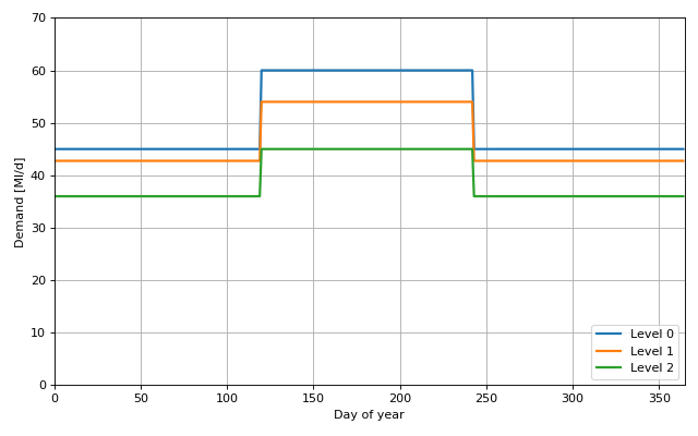
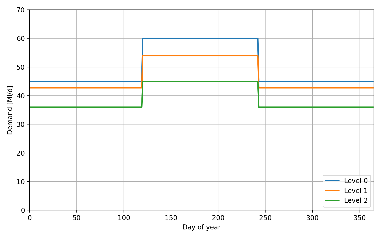
The final profiles are illustrated in the figure below. The actual demand value will switch between the three profiles depending on the resource state of the reservoir.
(Source code, png, hires.png, pdf)

This parameter can then be applied to the max_flow attribute of the demand node.
{
    "type": "output",
    "name": "Demand",
    "max_flow": "demand_max_flow",
    "cost": -500
},
When a model has more than one demand node it is OK to re-use the demand restriction level/factor for each demand node. Pywr will only calculate the index once for each parameter. Therefore, it is more efficient to share IndexParameter where possible.